Explaining Sentiment Scores With Transformers and SHAP

An example of what we’ll be doing in this article:

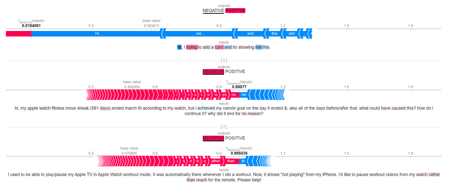
Wouldn’t sentiment analysis be made easier if we could find a way to show which terms or chunks of terms within a given corpus contribute to the overall sentiment score of the corpus or some of its parts?

I recently came across this pretty neat library named SHAP which amongst many other things provides some useful tools for explaining sentiment scores.

Sounds great to you too? Well let’s get going then!

I want to speak to your manager

If like me you have worked for a customer facing company, you probably know how difficult it is to obtain positive feedback on any of the products or services that you’re selling. If your Wi-Fi box suddlenly stops working, you’re very likely to take your phone and either call or tweet your internet access provider. However, I doubt you’re ever going to reach out to their customer service and tell them “Hey folks, my Wi-Fi is working perfectly today, great job on that!”.

Where are we going to find tweets that can be either positive, negative, or neutral you may wonder? A quick online search returned an article entitled the “Top 10 companies known for great customer service” and guess who came first? Apple, a company that I personally neither like nor dislike. Again, I have no idea as to whether that claim is true or not, but we don’t really care. All we want to do is obtain some data to play around with. And to get that, we’re going to use the following two libraries:

• SNScrape: We could, and probably should be using Tweepy to retrieve a list of recent tweets instead. But SNScrape also works with Facebook and a few other online social media networks so I highly encourage you to get familiar with it. Either way, please feel free to check out my article here if you want to get some practical exposure as to how Tweepy works.

• Tweet-Preprocessor: We’re lazy. So enough of that regular expressions non-sense, we’ll leave Tweet-Preprocessor to do all the cleaning for us. I also wrote an article that showed the potential of this text processing utility, in case you’re interested.

Let’s start by scraping the 500 most recent tweets sent to @AppleSupport on Twitter:

import snscrape.modules.twitter as sntwitter
import pandas as pd

def getTweets(handle,howmany):
    struct = {
        "Posted": [],
        "From": [],
        "Tweet": []
    }
    tweets = sntwitter.TwitterSearchScraper(f"{handle} lang:en").get_items()
    for i,t in enumerate(tweets):
        if i > howmany:
            break
        else:
            struct["posted"].append(t.date)
            struct["from"].append(t.user.username)
            struct["tweet"].append(t.rawContent)
    dframe = pd.DataFrame(struct)
    return dframe

getTweets("to:@AppleSupport",500)

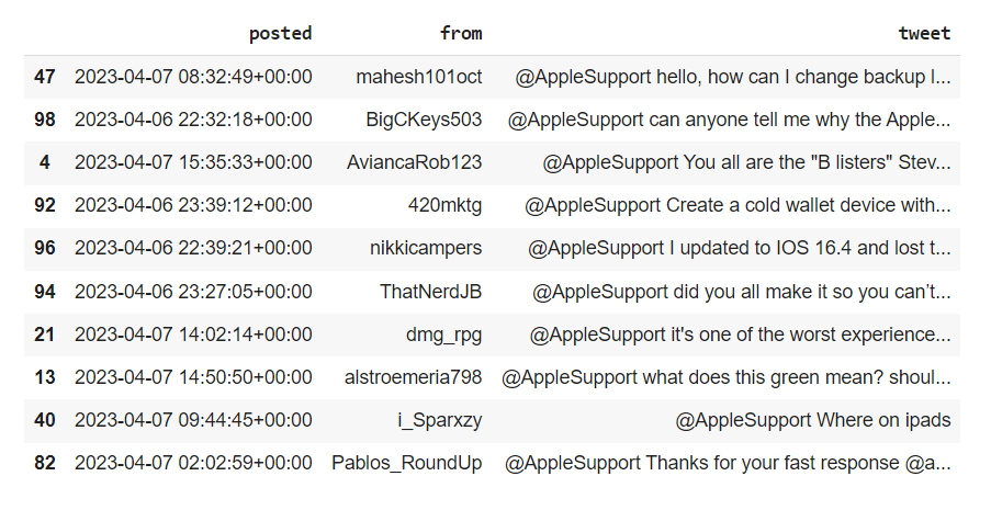
To be fair we only need to keep the Tweet serie, so let’s get rid of the remaining series that we no longer need:

df = df.filter(["Tweet"])

Alright, what’s important now is to clean this Tweet serie using Tweet-Preprocessor. We should now have a similar serie, but without any hashtag, emoji, urls, or mentions of any Twitter handle:

import preprocessor as p

df["cleaned"] = df["tweet"].apply(lambda x: p.clean(x))
df.filter(["cleaned"]).sample(10)

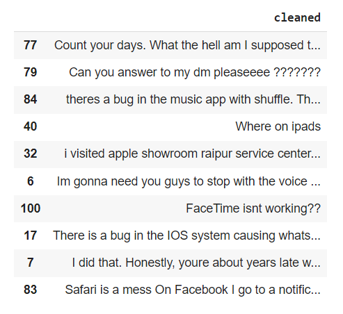
And we’re good to go!

An overview of the sentiment analysis landscape

Sentiment analysis has been around for a very, very long time. Funnily enough, some guy I used to work with had developed an interesting theory around what he called “repeated emotional signals”. Simply put, he had noticed that when people repeat the same punctuation sign more than twice, they’re usually not too happy. I have to admit that it worked surpisingly well with sarcasm, and we used his approach with relative success for while when writing some SQL queries:

• “Still haven’t heard back from you. What the hell are you guys doing???”
• “My debit card was supposed to arrive by post by EOD yesterday but still no sign of it. Hope you’re proud of youselves, my weekend is ruined..”
• “Is that really all you can do!!!”

The history of sentiment analysis closely follows that of natural language processing. We first went from the good old days of rule-based term-to-score matching to more statistical approaches. And since 2017 we’ve ditched all of that in favor of neural networks, because attention is everything.

But before into we dig into more modern and arguabbly more complex approaches, let’s take a closer look at what we mean by rule-based term-to-score matching. Most of the existing implementations are based on the Valence criterion, a subjective evaluation framework for emotions related to an event, object, person, or whatever else you want to.

If you have used NLTK the term VADER (Valence Aware Dictionary for Sentiment Reasoning) will for instance probably seem familiar to you. Another popular Valence-based lexicon is called AFINN, and its term / score matching system looks like this:

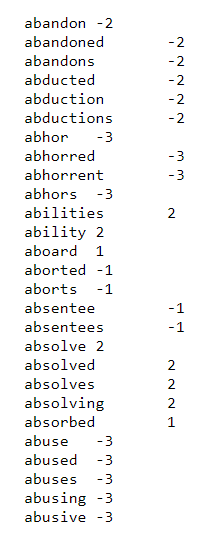
Implementing a rudimentary AFINN-based analyser in just a few lines of code is fairly easy:

def getSentiment(corpus):
    struct = {}

    with open("AFINN-en-165.txt", "r") as file:
        for f in file.readlines():
            struct[f.split("\t")[0]] = f.split("\t")[1].strip("\n")

    for t in corpus.split(" "):
        if t.lower() in struct:
            print(f"{t:<15} =>\t{struct[t]}")
        else:
            print(f"{t:<15} =>\t0")

text = "Hi, my name is Julien I love pizzas but I absolutely hate cauliflower"
getSentiment(text)

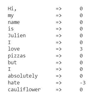
Now you might be wondering why would anybody use a rule-based approach for sentiment analysis in 2023? Well, first thing is, as we’re not using any model but simply matching an array of terms against some arbitrary scores, doing so is quite fast. But most importantly, not every company allows their data folks to install and use any framework or piece of software that they want to. If you work for a bank or an insurance company, you’re going to get access to a SQL engine, Excel, Matlab if you’re lucky, and that’s it. Forget about pip install-ing some fancy and modern libraries because you won’t be allowed to go ahead and do that. I know a few guys who still have to export the result of their SQL queries to a csv file, and then use Excel to try and compute some primitive sentiment score. Rock n’ roll.

Which leads us to the so-called workhorse of modern natural language processing, the transformers architecture. They have progressively replaced recurrent neural networks for text processing tasks, like summarisation, translation, classification, etc.. Tranformers handle large sequences better and are pretty good at parallelizing which makes them easier to train. I won’t pretend that I can explain the transformers architecture better than the resources that I’m about to share (which probably means that I don’t understand how they work as well as I think I do!), so before I start making a fool of myself I strongly suggest that you check out the following articles:

• Transformers in NLP: a beginner-friendly explanation
• How do Transformers work?

At our modest level, all that we need to know is that transformers focus heavily on:

• Attention: Technically speaking, an attention mechanism is a layer in a deep neural network. More simply put, transformers process sequences of vectorised terms. For each layer, these sequences are then “transformerd* into another sequence of vectors, called hidden state. Right, but why do we care? Well, this is a major improvement over word2vec or GloVe, as this time the attention mechanism considers all the words in a sentence when creating a word embedding for a given word. Which in turn means that the same word that is used in two or more sentences will have a word embedding that is specific to each sentence. Actually, self-attention is the real show-stealer here. It is through self-attention that transformers try to determine how words in a sentence are interconnected with each other.

• Positional encoding: The position of each term within a given sentence is stored directly within the data, and not within the model. Why this matters is that it allows the model to learn the importance of the positioning of each term.

If you’re more into videos than into research papers and articles, then this short introductory presentation does a pretty decent job at explaining the basic concepts of the transformers architecture:

What makes this whole field look more confusing that it actually is, is that there exist at least a dozen various implementations of the original transformers architecture. So before we move on to some practical examples, let’s take a quick look at the two models that we’ll be experimenting with today. Both are based upon Google’s 2018 BERT model, and modify some of its key hyperparameters:

• RoBERTa was developed in 2019 by two Facebook employees and implemented in PyTorch. It was trained with much larger mini-batches and learning rates, and improves on BERT’s language masking strategy across a variety of natural language processing tasks.

• DistilBERT stands for distilled BERT and for developed in-house at Huggin Face in 2019. According to its authors, DistilBERT “has 40% less parameters than bert-base-uncased, runs 60% faster while preserving over 95% of BERT’s performances as measured on the GLUE language understanding benchmark”.

With this out of the way, it’s finally time for us to start playing around with the tweets that we scraped earlier on.

A love / hate relationship

Our plan here is simple: we process tweets through each model, output a sentiment score, and then briefly investigate any discrepency within our results. Please note that the Python code that we’ll be writing in this section is poorly optimized. We should refrain from using Pandas’s .apply() method, and go for vectorization instead of for loops whenever possible. That being said, performance and optimization aren’t what’s being discussed in this article.

• For the good old rule-based approach, we’re naturally going to use NLTK, a popular library that amongst many other things offers a reliable implementation of the Valence criterion. Here’s how:

import nltk
from nltk.sentiment.vader import SentimentIntensityAnalyzer

text = "I also hate artichokes"

sia = SentimentIntensityAnalyzer()
result = sia.polarity_scores(text)

for k,v in result.items():
    print(f"{k:<10} =>\t{v}")

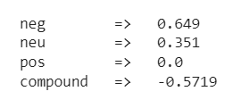
We get a dictionary that contains a negative, neutral, and positive score, plus something called compund, that basically sums the three values and normalizes them.

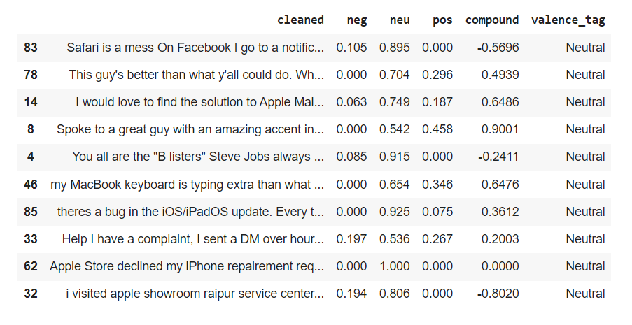
To transform all of this into a Pandas dataframe as well as add another serie that takes the highest value within our dictionary and outputs a correspondinf tag categorical value, we can write the two following functions:

def getSentiment(data,serie):
    sia = SentimentIntensityAnalyzer()
    sentiment_cols = {}
    for i,col in enumerate(data[serie]):
        sentiment_cols[i] = sia.polarity_scores(col)
    sentiment_df = pd.DataFrame(sentiment_cols)
    return sentiment_df.T

def getSentimentTag(data):
    result = []
    for i,v in data.iterrows():
        scores = [v[1],v[2],v[3]]
        m = max(scores)
        ind = scores.index(m)
        if ind == 0:
            result.append("Negative")
        elif ind == 1:
            result.append("Neutral")
        else:
            result.append("Positive")
    return result

sent_valence = getSentiment(df,"cleaned")
valence = pd.merge(df["cleaned"], sent_valence, left_index=True, right_index=True)
valence["valence_tag"] = getSentimentTag(valence)
valence.sample(10)

We’ll be implementing a similar logic to process our tweets using RoBERTa, but let’s see first how to output a sentiment score for a simple sentence. We start by importing the necessary modules, and by picking a model:

from transformers import AutoTokenizer
from transformers import AutoModelForSequenceClassification
from scipy.special import softmax

tokenizer = AutoTokenizer.from_pretrained("cardiffnlp/twitter-roberta-base-sentiment")
model = AutoModelForSequenceClassification.from_pretrained("cardiffnlp/twitter-roberta-base-sentiment")

We then copy and paste the code that can be found directly on Huggin Face’s website and slightly modify it so that it processes our simple sentence:

text = "Actually, I hate vegetables in general."

encoded_text = tokenizer(text, return_tensors="pt")
output = model(**encoded_text)
scores = output[0][0].detach().numpy()
scores = softmax(scores)

for s in scores:
    print(s)

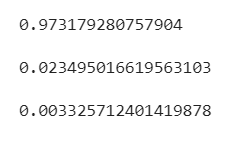
If you’re wondering what SciPy’s softmax() function does, here’s what we can read on the official website:

“The softmax function transforms each element of a collection by computing the exponential of each element divided by the sum of the exponentials of all the elements. That is, if x is a one-dimensional numpy array”

We get this time a list, with its elements corresponding to negative, neutral, and positive values respectively. Just like we did earlier on when using NLTK, we can create two separate functions to process our tweets and unpack the resulting sentiment arrays:

def getSentimentRoberta(data,serie):
    sentiment_cols = {
        "neg" : [],
        "neu" : [],
        "pos" : []
    }
    for i,col in enumerate(data[serie]):
        encoded_text = tokenizer(col, return_tensors="pt")
        output = model(**encoded_text)
        scores = output[0][0].detach().numpy()
        scores = softmax(scores)
        sentiment_cols["neg"].append(scores[0])
        sentiment_cols["neu"].append(scores[1])
        sentiment_cols["pos"].append(scores[2])
    sentiment_df = pd.DataFrame(sentiment_cols)
    return sentiment_df

sent_roberta = getSentimentRoberta(df,"cleaned")
roberta = pd.merge(df["cleaned"], sent_roberta, left_index=True, right_index=True)
roberta["roberta_tag"] = getSentimentTag(roberta)
roberta.sample(10)

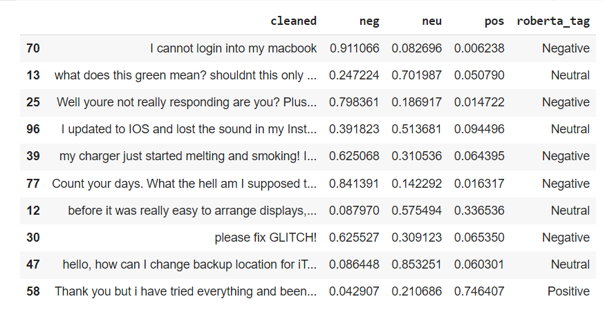
Finally, let’s add a “mismatch” serie to our dataframe and go through some of the tweets that our two models might be disagreeing about:

def getMismatch(data):
    result = []
    for k,v in data.iterrows():
        if v[1] == v[2]:
            result.append(False)
        else:
            result.append(True)
    return result

def combineSentiment(left,right):
    l = left.filter(
        ["cleaned","valence_tag"]
        )
    r = right.filter(
        ["cleaned","roberta_tag"]
        )
    combined = l.merge(
        r,
        how="left",
        left_on="cleaned",
        right_on="cleaned"
        )
    return combined

mismatch = combineSentiment(valence,roberta)
mismatch["mismatch"] = getMismatch(mismatch)
mismatch.query('mismatch == True')

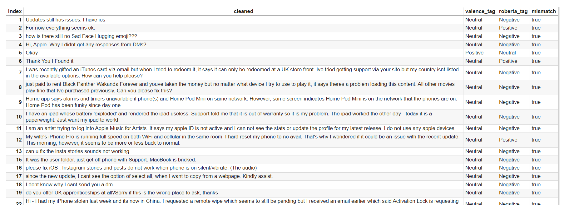
Overall, roBERTa seems to be providing much more accurate results, as well as more balanced spread of sentiment tags. We can easily confirm this by plotting the distribution of scores for both models:

from collections import Counter
import plotly.graph_objects as go
from plotly.subplots import make_subplots
import plotly

def getCount(serie):
    result = {
        "tag": [],
        "volume": []
    }
    c = Counter(serie)
    for k,v in c.most_common():
        result["tag"].append(k)
        result["volume"].append(v)
    return result   

def getDoubleBarPlots(x1, y1, x2, y2, title, subtitle1, subtitle2):
    cols = ["#003f5c","#bc5090","#ffa600"]
    fig = make_subplots(rows=1, cols=2, subplot_titles=(subtitle1, subtitle2))
    fig.layout.template = "plotly_white"
    fig.add_trace(
        go.Bar(
            x=x1,
            y=y1,
            orientation="h",
            marker_color=cols,
            width=0.8,
        ),
        row=1,
        col=1,
    )
    fig.add_trace(
        go.Bar(
            x=x2,
            y=y2,
            orientation="h",
            marker_color=cols,
            width=0.8,
        ),
        row=1,
        col=2,
    )
    fig.update_layout(
        title=title,
        bargap=0.01,
        showlegend=False,
        template="plotly_white",
        plot_bgcolor="#E9E8E8",
        paper_bgcolor="#E9E8E8",
        width=900,
        height=450,
        font=dict(
            family="Arial",
            size=18
        )
    )
    fig.update_yaxes(
        type="category",
        categoryorder="total ascending"
        )
    fig.show()

valence_tags = getCount(mismatch["valence_tag"])
roberta_tags = getCount(mismatch["roberta_tag"])
getDoubleBarPlots(
    valence_tags["volume"],
    valence_tags["tag"],
    roberta_tags["volume"],
    roberta_tags["tag"],
    "Sentiment tags distribution","Valence","roBERTa"
    ) 

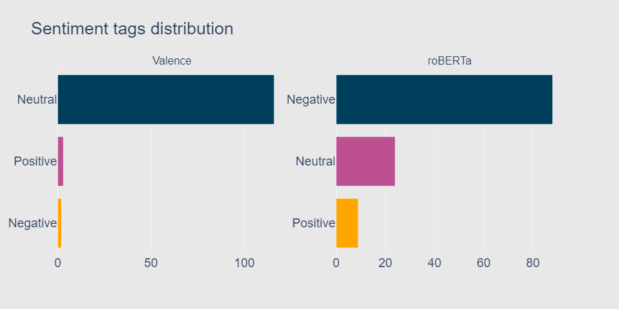
Ok that’s not too bad, but none of these charts show us how the sentiment scores for each tweet are determined. Wouldn’t it be better if we could visualise what specific terms or parts of a sentence play a role in how the values are computed?

I have some scores, what do I do next?

Dear readers, this is exactly what the SHAP library is going to do for us. But before we jump into some practical examples, let’s head over to the official website and see what this great package is all about:

“SHAP (SHapley Additive exPlanations) is a game theoretic approach to explain the output of any machine learning model. It connects optimal credit allocation with local explanations using the classic Shapley values from game theory and their related extensions.”

In other words, it uses Shapley values to explain the output of pretty much any machine learning model. More specifically, SHAP provides a series of tools to help understand and debug the following models:

• Tabular data: Tree-based, linear, and agnostic models, plus neural networks
• Text: sentiment analysis, translation, text generation and summarization, as well as question-answering
• Images: classification and captioning

As you can see, the list of features and visualisations that this library supports is quite compehensive. Though going through each of the aforementioned spaces would probably be fun, I don’t intend to write a Tolstoi-long article either, so we might want to limit ourselves to their sentiment analysis page for now and see what’s in there.

Though we should probably stick to the examples that they provide first, we’ll see if we can add a personal touch to their base code. For now let’s import the base libraries:

import transformers
import shap
import numpy as np

Remember earlier when we briefly discussed what DistilBERT is? We’re going to initialise our transformers model and simply leave the first parameter for the .pipeline() class as default (in our case, “sentiment-analysis”):

classifier = transformers.pipeline("sentiment-analysis", top_k=None)

Which immediately leads to the following warning message:

“No model was supplied, defaulted to distilbert-base-uncased-finetuned-sst-2-english and revision af0f99b”

And that’s perfectly fine for today, but feel free to check here if you want to see a whole list of models that can be used instead. Anyway, we need to feed a list of strings to our classifier() instance. Doing so can be achieved by using Pandas’s built-in to_list() method, and for now we’re only going to take the first three tweets. Now if we weren’t lazy, we would probably be using a sentence vectorizer instead. But that’ll do for today:

test_df = df["cleaned"][:3].to_list()

for cl in classifier(test_df):
    for c in cl:
        print(c)

We fed this list of strings to our transformers pipeline, and in return we got a sentiment classification as well as a sentiment score for each of our individual array element.

The SHAP library processes the output of any given model through what is called an “explainer”. To instantiate the “explainer”, we simply call the .Explainer() function and feed as its first argument the model that we chose earlier:

explainer = shap.Explainer(classifier)
shap_values = explainer(test_df)
print(shap_values)

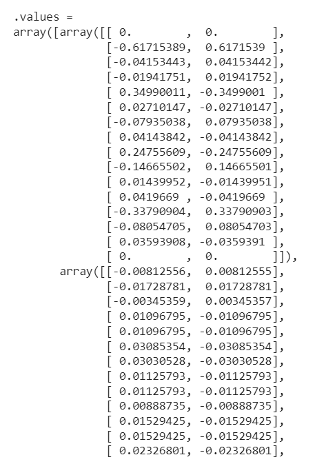
As you can see in the screenshot above, we get nested arrays representing the sentiment score for our first three tweets, because we earlier on passed the transformers.pipeline("sentiment-analysis", top_k=None) model as an argument. Had we had numerical values and not text, we would of course have chosen a different model.

print(type(shap_values))

Alright, we can now try to explain our first three tweets using SHAP’s built-in .plots.text() method:

def getTextPlot(data):
    shap.plots.text(
        data,
        xmin=-0.1
        )

getTextPlot(shap_values)

And we get this very interesting multi-level visualisation, where the positive and negative elements of each tweet are outlined in either blue or red depending on their polarity. The upper-part color-scale maps the most positive and negative terms, positioned relatively to their individual score. Beneath this is the full tweet, with its strong positive and negative terms colored accordingly. You’ll see that I have limited the minimal value of the x-axis to -1, but this is entirely optional.

While this first visualisation is already pretty useful, it can quickly become difficult to read if we’re using textual data that’s longer than a few sentences. To circumvent this, we can either use a sentence tokenizer, and loop through each sentence. Another approach is to use SHAP’s .plots.bar() method, which shows which terms or combinations of terms have a strong sentiment score:

def getBarPlot(data):
    shap.plots.bar(
        data,
        order=shap.Explanation.argsort,
        clustering_cutoff=1
        )

getBarPlot(shap_values[0,:,"POSITIVE"])

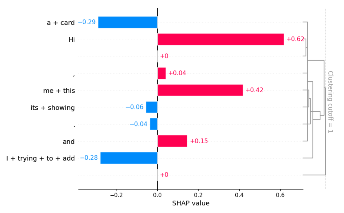
As you can see, we told SHAP that we wanted to sort our terms by their sentiment score, and we then passed shap_values[0,:,"POSITIVE"] into our function. Please note that we could have passed shap_values[0,:,"NEGATIVE"] instead, which would have reversed the polarity of the colorscale.

We can also slightly amend the output by passing the mean of our values instead:

def getBarPlot(data):
    shap.plots.bar(
        data,
        order=shap.Explanation.argsort
        )

getBarPlot(shap_values[:, :, "POSITIVE"].mean(0))

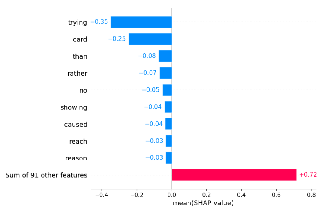
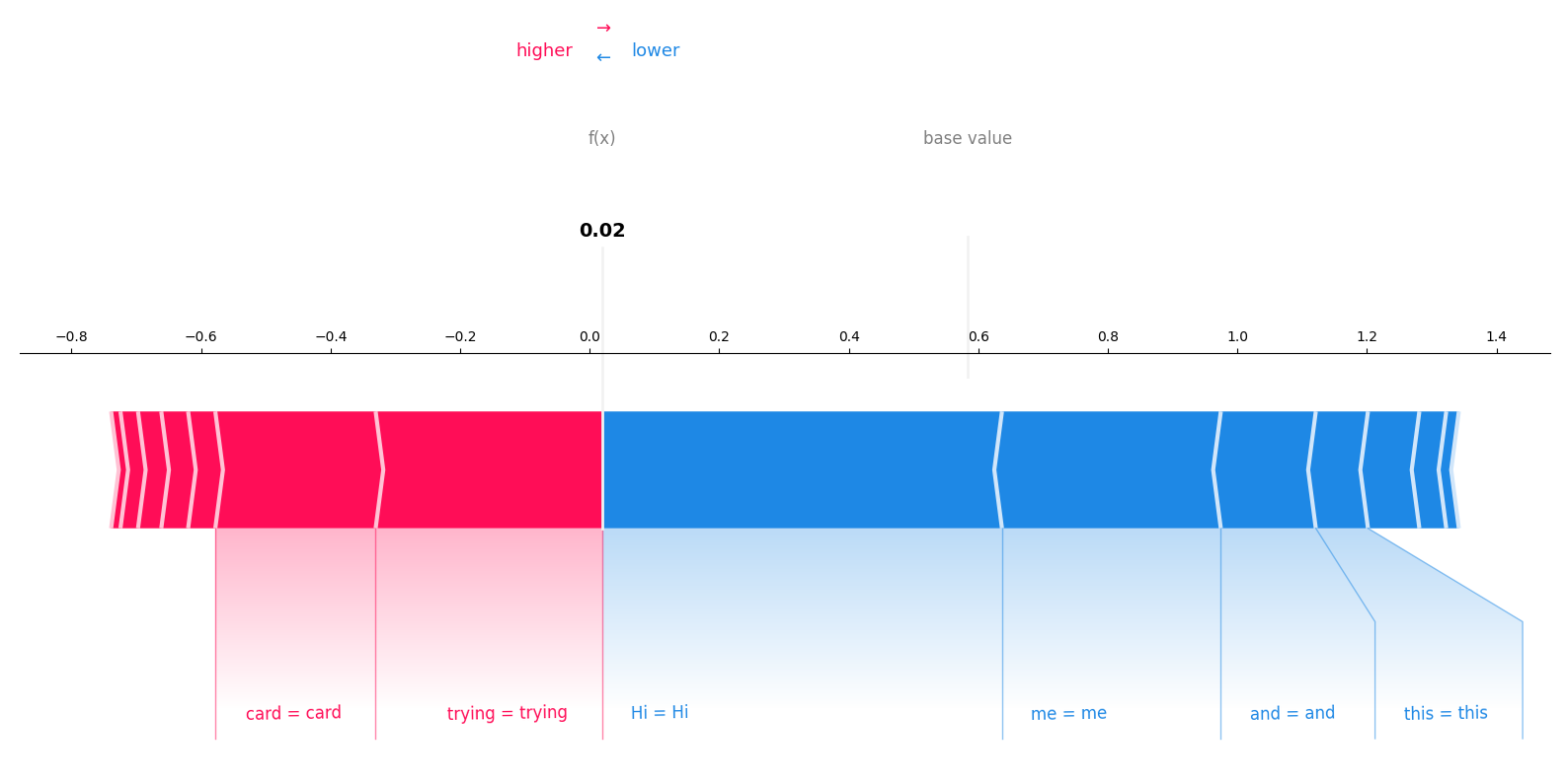
Finally, SHAP features this .plot.force() method, which allows for more aguments, like for instance the possibility to generate the visualisations using Matplotlib as a wrapper. This then allows us to manually set the size of the figure, choose a colormap, save the output to a file, etc..:

def getForcePlot(data):
    shap.plots.force(
        data,
        matplotlib=True,
        figsize=(20,6),
        plot_cmap=["#77dd77", "#f99191"],
        text_rotation=1
    )

getForcePlot(shap_values[0,:,"NEGATIVE"])

There’s much more to discover here, and I strongly encourage you to also try using SHAP with data types other than text. This library has a huge potential and can definitely help you better understand the outputs of your models, and is to me a game-changer for machine learning explainability.